User notes for R&K Langmuir trough users

Contents
• overview and specifications
• acknowledgments
• unpacking and mounting the trough
• cleaning the trough and glass block
• vibration isolation
• interfacing with the trough and controling it
• controling the trough via computer
• trough calibration
• constant pressure mode
• isotherm macro

See also:
• notes from Elaine Dimasi for the trough at Brookhaven X22-B.
• documenatation from Riegler and Kierstein
• Instructions for the surface pressure transducer
• schematic of the surface pressure circuit
• schematic of the barrier motor drive circuit
• schematic of the pressure/area command circuit

The CMC trough comes in two boxes, a large one containing the trough canister and a smaller one containing the trough itself, the control unit, the connecting cables and a box with various accessories. We have recently fitted the trough canister with spacer plates to position the trough higher in the canister and thereby decrease the time necessary to fill the trough with helium. (Before you put the trough into the canister, it's a good idea to clean it under the hood in the lab.) The levelling feet on the trough fit into depressions in the top spacer plate. Make the connections between the trough and the waterbath hoses and the control box cable feedthroughs. In the cardboard accessory box, find the surface pressure transducer, mount it on the post on the trough, and connect the wires. Hang the Wilhelmy plate and hook from the plastic loop on the transducer. 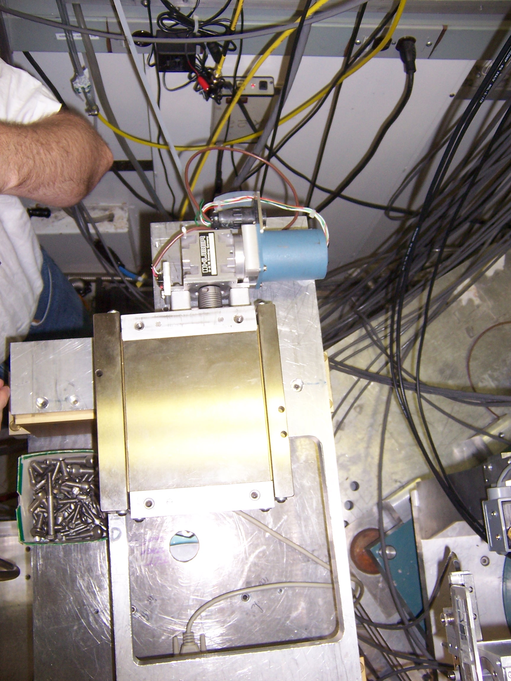Mount the canister and the trough on the sample stage. The foot of the canister near the window should be approximately centered on the center of the sample theta, two-theta rotation stages. The other two feet, along with a fair amount of the canister, will hang over the side of the sample stage's adapter plate. Make the connections between the canister feedthroughs and the circulating bath and the control box cables. 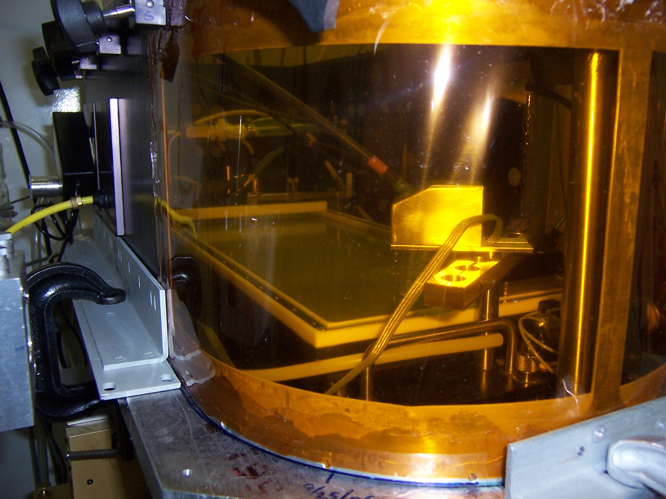Level the trough using the three adjustable feet on the trough. Put the (clean) glass block into the trough and fill the trough with water.

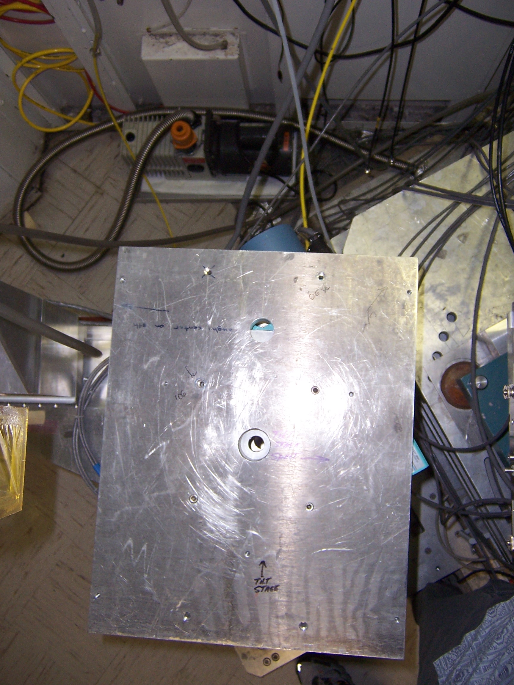
At X22-B, you may have to mount the trough after an experiment not requiring the trough. There is hardware at the beamline that holds the trough in place. (The plates are stored in the X22 cabinet, along with the anti-vibration stages. The dogs for the anti-vibration stages are in the cabinet in the hutch. The screws and bolts are in a green cardboard box in the hutch. The anti-vibration controller and cables are beneath the table holding the 4-circle. ) See the photos below.

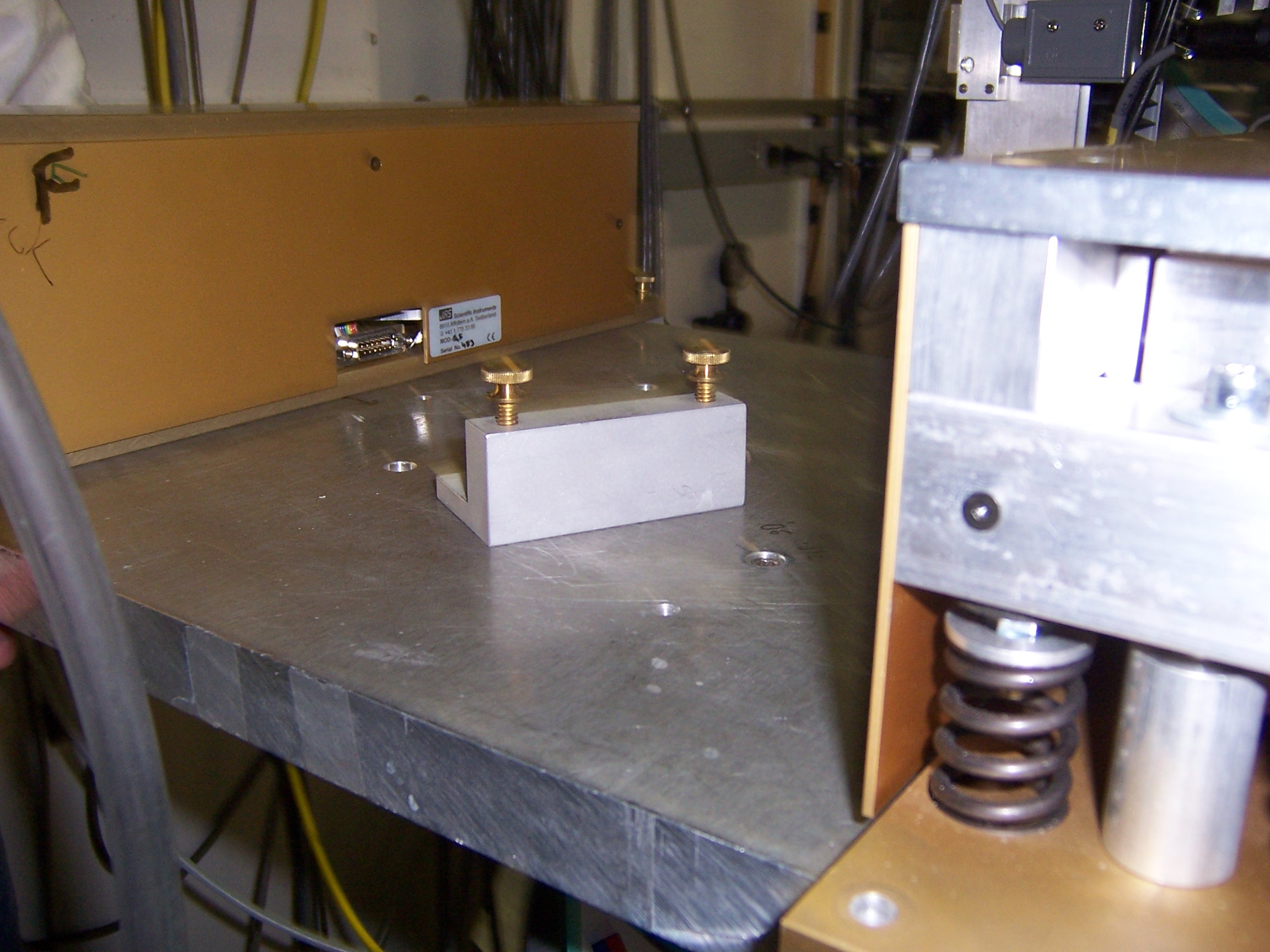
The base plate was centered on the sample stage for the previous experiment.	To mount the trough, the base plate must be offset from the center.
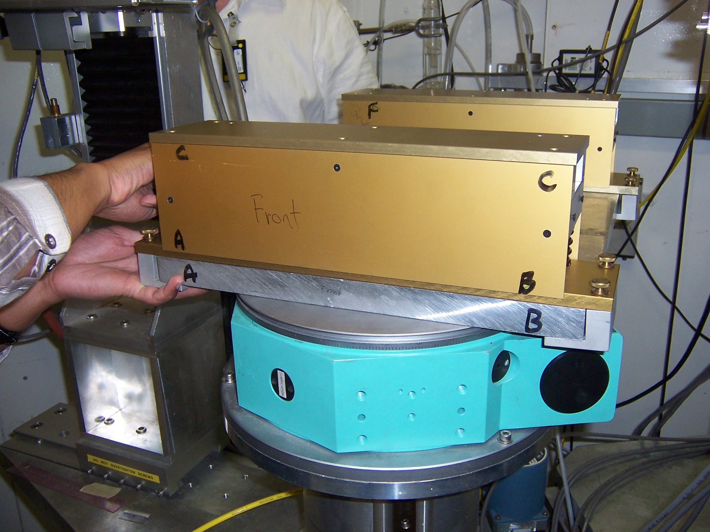
The anti-vibration stages hang over the edge of the base plate and are secured with dogs. Keep the dogs loose until the other components are also in place.	The letters marked on the plate and anti-vibration stages ensure the correct alignment of the components.
The adapter plate is secured by only 3 screws to each anti-vibration stage.	The translation state goes on next. It has spacer plates installed so that no washers are necessary. The trough base plate goes on next, and then the dogs on the anti-vibration stages can be tightened.
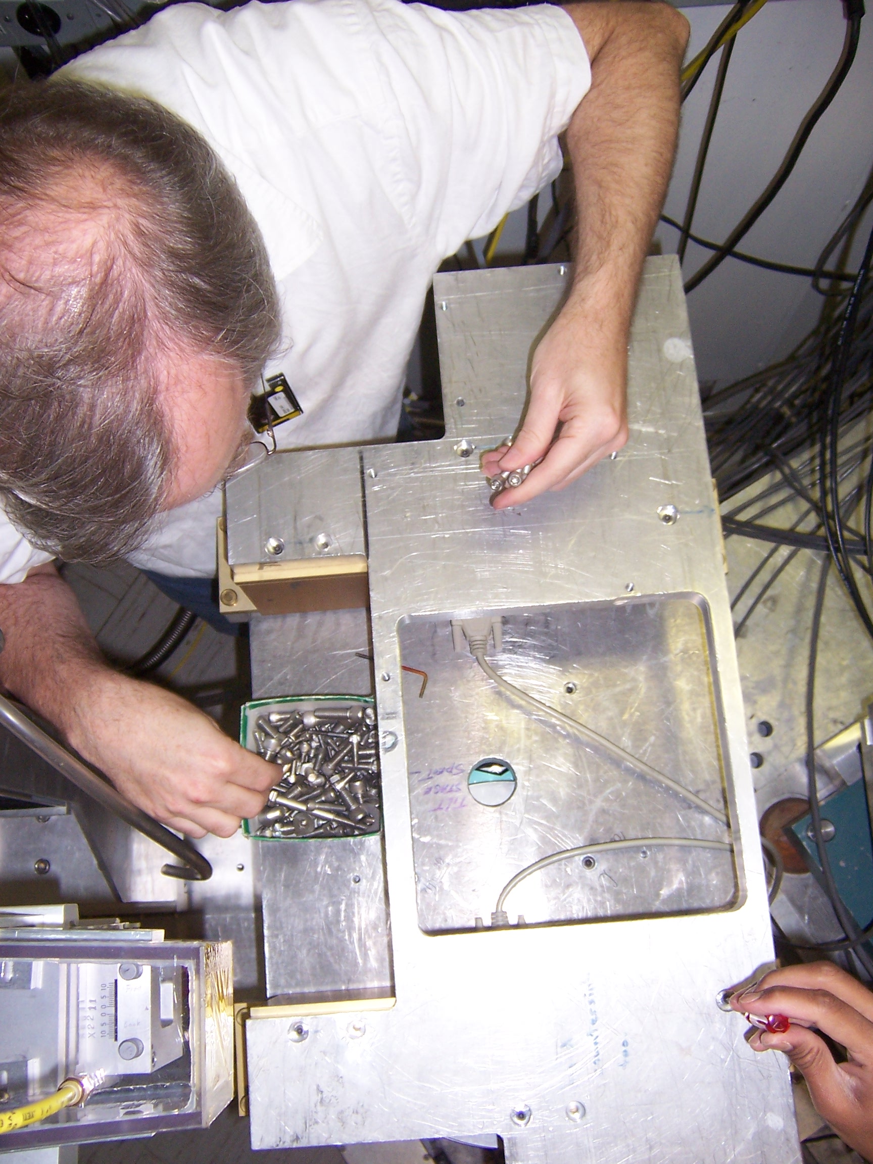
The outline of the trough is marked on its base plate. Use c-clamps and metal pieces to secure the trough in position.

top

Cleaning the trough and glass block

Sometimes the trough needs to be cleaned more thoroughly, for example when the next sample is very different, or requires a different subphase, or if the previous monolayer's meniscus collapsed and contaminated the teflon edges of the trough. Aspirate the monolayer carefully as just described, then take out the block from the subphase and either put it aside (best to keep it covered with clean water) or clean it. Then aspirate the subphase completely and wipe down the trough and barrier as necessary, paying careful attention to any hydrophilic patches you may have noticed. Be extra careful using solvents in the hutch. Transfer a few milliliters to clean vials for use in the hood. You don't need much to clean the trough. Collect the contaminated Kim-Wipes and your gloves for disposal. Fill the trough with clean water and aspirate it out a few times before returning the block to the trough and adding the subphase for the experiment.
top

Vibration Isolation

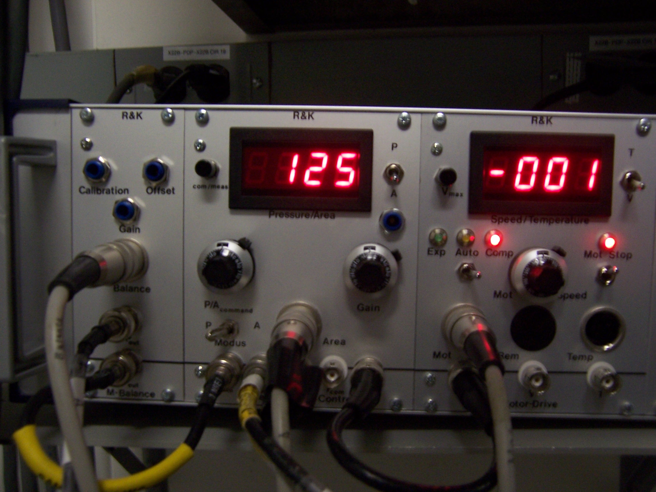
The trough control unit consists of three modules, as seen in the above picture. From left to right we see the Pressure, Area and Barrier modules. The Pressure module has three trimpots that affect the pressure calibration and offset, and the gain of the transducer. The area module has an LED display that displays pressure or area, depending on the setting of the togggle switch to the right of the display. Additionally, depressing the pushbutton to the left of the display switches the readout from 'MEASure' mode (current pressure/area displayed) to 'COMmand' mode (the pressure/area setpoint is displayed). The display on the barrier module shows a number proportional to the velocity of the moving barrier or the temperature of the probe in the subphase of the trough, depending on the setting of the toggle switch to the right. It contains the switches for moving the barrier manually or engaging constant pressure mode. The knob below the display determines the barrier speed.

Connect the trough control unit to power and connect all the cables from the trough. Use short coax cables from the cardboard accessory box to connect the P_out terminal from the Pressure module to the P_in terminal on the Area module and the S_out terminal of the Area module to the S_in terminal of the Barrier module. Now the control unit can read out the total area of the monolayer, the surface pressure and the temperature. To record pressure-area diagrams, interface the control box with the computer running Surf. The details are different for CMC CAT and X22B. At X22B, connect the P_out terminal to the digital multimeter (labelled GPIB 03) located above the computer terminal via the patch panel in the hutch. Similarly, connect the A_out terminal to the DMM labelled GPIB 05. The macro below will tell Surf how to read in the data. (Note that without a third DMM, there is no provision for reading in the temperature from the probe in the subphase. However, the NESLAB chiller can be computer-interfaced so that the bath temperature can be recorded. See Elaine Dimasi's notes for the chiller unit on her LSS documentation page.) At CMC CAT, the P_out, A_out and T terminals should be connected to voltage to frequency converters (VFC) in the B-Hutch and the output connected to scaler channels. See the information in the macros section for more details.

top

Computer-Interfaced Control of the Trough

Pi calibration The filter paper used as the Wilhelmy plate should be 3 mm wide and should extend approx. 12 mm from the hole for the hook. For a coarse, but generally reliable, calibration:

• with the paper in the water, adjust the potentiometer labeled "offset" to zero
• Move the balance head so the paper is out of the water
• Adjust the potentiometer labeled "calibration" so the pressure display reads 72.
• Note the voltage readings with the paper in and the paper out. You should observe 0.0 and 7.2 V.
• CMC: You need to set the scale factor so that the voltage is interpreted properly. From Spec, enter config, then adjust the scale factor for the appropriate scaler.
• X22B:You need to tell Spec how to interpret the voltage by setting the parameters PRESSURE_OFFSET and PRESSURE_SLOPE. From the command line, enter PRESSURE_OFFSET=0 and then PRESSURE_SLOPE=10. Or you could change the values in your copy of the isotherm macro and then do the macro again. (If these parameters are undefined in Spec, you need to run the macro to set things up).

Generally speaking, this calibration is sufficient. You may want to test things out by taking an isotherm of a standard substance, like arachidic acid.

top

Area calibration It is possible to adjust the offsets of the electronics so that the area signal is proportional to the total area of the trough, but the procedure is cumbersome. It is more convenient to set the calibration in the software instead. Both troughs are exactly 16 cm wide. Use a ruler and measure the distance from the barrier to the front end of the trough for two different points and record the voltage of the area signal at each position. The area signal is very linear with barrier position, so from the two points you can derive the slope and y-intercept of the line through the two area-voltage pairs.

• X22B: In Spec, set the value of the parameters AREA_OFFSET and AREA_SLOPE according to your calibration equation. (see the X22B note in Pi calibration)
• CMC: When you plot the isotherm data, use your equation to transform your data. In config mode, choose a scale factor for the area scaler that gets things approximately correct, then just use be sure to apply your calibration equation to the area data when you plot your isotherms.

The constant pressure mode of the trough controller allows you to compress the monolayer to a set pressure (or area) that you determine and then maintain the monolayer at that pressure (or area). (The area control is intended for different troughs with two moving barriers.) To set the target pressure (0) check that the toggle switch at the bottom of the middle module (modus) is in the P position; (1) look at the LED display on the moddle module and make sure that the toggle switch on the right side is set to pressure (P); (2) depress the pushbutton (com/measure) to the left of the display; the LED display now shows the target pressure; (3) turn the knob at the lower left of the display (P/A command) until the desired target pressure is displayed. To engage constant pressure mode (1) check that the toggle switch on the right side of the right module (mot stop) is in the up position and the LED is lit; (2) put the three-way toggle switch on the left side of that module (exp auto comp) into the auto position; (3) as soon as you toggle the (mot stop) switch to the down position, the monolayer will be compressed until the target pressure is achieved. The Gain knob on the middle module controls the characteristics of the feedback loop that moves the barrier. To disengage constant pressure mode toggle the mot stop switch to the up position and stop the barrier motion, or put the three-way switch into the exp or comp position, which will immediately start expanding or compressing the monolayer.

top

Isotherm Macros

global  PRESSURE        # last pressure reading  			
global  PRESSURE_SLOPE  # linear coefficient for pressure reading	
global  PRESSURE_OFFSET # constant term for pressure reading	
global  AREA            # last area reading			
global  AREA_SLOPE      # linear coefficient for area reading	
global  AREA_OFFSET     # constant term for area reading	
global  DEGC            # temperature				
global  ISO_GROUP       # group number for isotherm data (choose 7)

PRESSURE_SLOPE = 10							
PRESSURE_OFFSET = 0							
#####March 2001 values for correctly calibrated trough (readout		
#####on control unit is accurate					
AREA_SLOPE = 109.7							
AREA_OFFSET = -1.2464							
ISO_GROUP = 7								

def getpia '								
        PRESSURE=gpib_get(3)*PRESSURE_SLOPE+PRESSURE_OFFSET		
        AREA=gpib_get(5)*AREA_SLOPE+AREA_OFFSET				
        '								

def press '								
        getpia								
        print "Pressure = ", PRESSURE, "\tArea =", AREA			
        '								

#measure1 is called from the "scan_loop" in the standard macros		
def measure1 '								
        getpia								
        '								

def iso_Fheader '_cols += 3;printf("#X %gKohm (%gC)\n", TEMP_SP,DEGC_SP)'  
def iso_Plabel  'sprintf("%7.7s %7.7s %8.8s ","Area","T-degC","Pressure")' 
def iso_Pout    'sprintf("%7.5g %7.5g %8.5g ",AREA,DEGC,PRESSURE)'	    
def iso_Flabel  '"Area  DegC  Pressure  "'				
def iso_Fout    'sprintf("%g %g %g ",AREA,DEGC,PRESSURE)'		
def iso_Ftail   ''							

        rdef Fheader "iso_Fheader"					
        rdef Plabel  "iso_Plabel"					
        rdef Pout    "iso_Pout"						
        rdef Flabel  "iso_Flabel"					
        rdef Fout    "iso_Fout"						
        rdef Ftail   "iso_Ftail"					

# this macro stuffs the scan data at each point of the scan		
# 9/26/98  Put in commands to fix plotting ranges--seems to work.	
def isoplot '								 
	_sx = _sx * 1.16 - 0.4						
        _fx = _fx * 1.16 - 0.4						
        data_put(ISO_GROUP, NPTS, 2, AREA)				
        data_put(ISO_GROUP, NPTS, 3, DEGC)				
        data_put(ISO_GROUP, NPTS, 4, PRESSURE)				
        X_L = "Area"							
        Y_L = "Pressure"						
	'								


def iso '								
        def _cleanup3   \'						
                PL_G = 0							
                PL_X = 0							
                PL_Y = 1							
                rdef scan_plot "_plot"						
                \'								
        rdef scan_plot "isoplot ; _plot"					
        data_grp(ISO_GROUP, 4096, 5)						
        PL_G=ISO_GROUP								
        PL_X=2									
        PL_Y=4									
         ascan sh A[sh] A[sh] 4000 1						
        '